Self-Taught Reinforcement Learning
In this project, I developed a small Reinforcement Learning library in Python. The goal was to learn the basics of RL by implementing the algorithms from scratch.
The documentation of the code has been made using Sphinx and the library is available on GitHub.
Here is the content of this page:
The Library
I wanted the library to be as simple as possible to use. The user only needs to define the environment and the agent, and then run the training loop on a Gymnasium environment, predefined in the library, or on a custom environment. For example, the following code trains a PPO agent on the BipedalWalker-v3 environment, where a 2D character must learn to walk:
from rlib.learning import PPO

env_kwargs = {'id': 'BipedalWalker-v3'}
agent_kwargs = {'hidden_sizes': [256, 256], 'activation': 'tanh'}

agent = PPO(env_kwargs, agent_kwargs)
agent.train()
By doing so, the user can solely focus on the implementation of the environment. The list of different algorithms available in the library is the following:
Q-Learning, where the Q-function is a table of size defined by the user.Deep Q-Learning, where the Q-function is approximated by a neural network. Does not handle continuous action spaces.Evolution Strategy, where an estimate of the gradient is computed using randomly sampled perturbations of the parameters. Handles both discrete and continuous action spaces.Deep Deterministic Policy Gradient (DDPG), where the policy is approximated by a neural network. Only handles continuous action spaces.Proximal Policy Optimization (PPO), where rather than optimizing the Q-function, the policy is optimized directly. Handles both discrete and continuous action spaces.
Results
We display here some results obtained with the library.
Q-Learning
We trained a Q-Learning agent on the MountainCar-v0 environment, where a car must learn to climb a hill. The agent was trained on 100,000 episodes and the following plot shows the evolution of the reward during training:
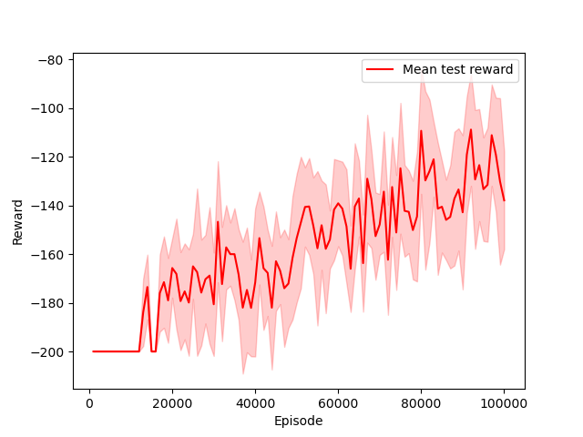
The reward here is the opposite of the number of steps before the car reaches the top of the hill, it is hence negative. We can see that the agent learns to climb the hill after about 10,000 episodes, and then improves its performance until the end of the training.
Here is a showcase of the training of the agent:
| Iteration 0 | Iteration 50,000 | Iteration 100,000 |
|---|---|---|
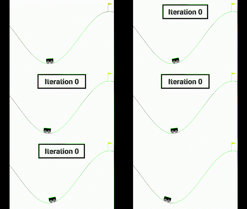 | 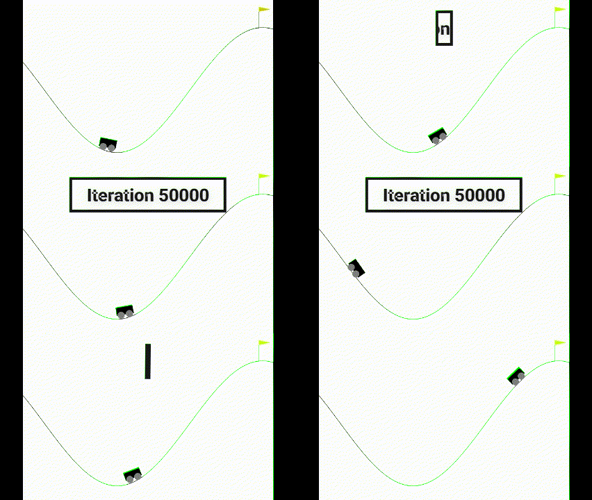 |  |
We can observe that the agent progressively learns how to climb the hill. It first learns how to swing to gain momentum, then learns how to reach the final flag.
Another interesting visualization is to plot the Q-function learned by the agent. This is possible has only two dimensions are needed to represent the state of the environment. By applying a softmax function on the Q-function, we can obtain a sort of probability distribution over the possible actions for each state. I.e. it shows how bigger or lower the impact of one action is compared to the others. The following plots show the Q-function learned by the agent after 100,000 episodes:
| Probability to go left | Probability to do nothing | Probability to go right |
|---|---|---|
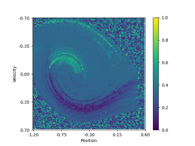 | 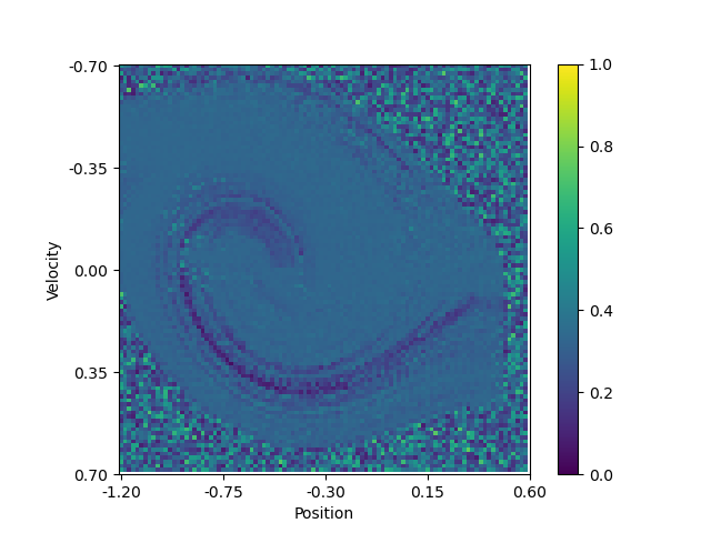 | 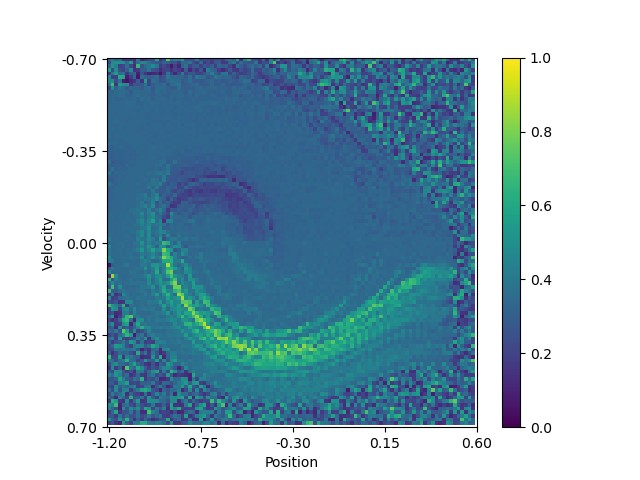 |
We can see a swirling curve on which the agent will move left or right. And that doing nothing is not a good option, as no area of the plot has a high value. Note that the pixelated areas are states where the agent has never been, or not often enough, to have a good estimate of the Q-function.
Deep Q-Learning
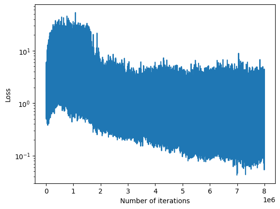
We trained a Deep Q-Learning agent on the LunarLander-v2 environment, where a small spaceship must learn how to land on a landing area. It has been trained on 500,000 environment steps and the following plot shows the evolution of the reward and loss during training:
| Test Rewards | Losses |
|---|---|
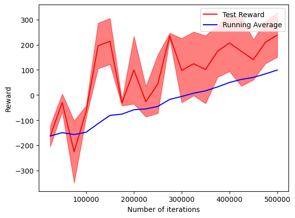 |  |
The agent manages successfully to train, achieving test rewards higher than 200 at the end of the training, which is the suggested success reward.
Here is a showcase of the training of the agent:
| Iteration 0 | Iteration 25,000 | Iteration 50,000 |
|---|---|---|
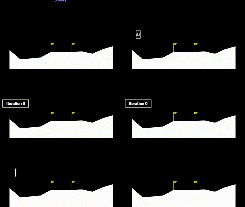 | 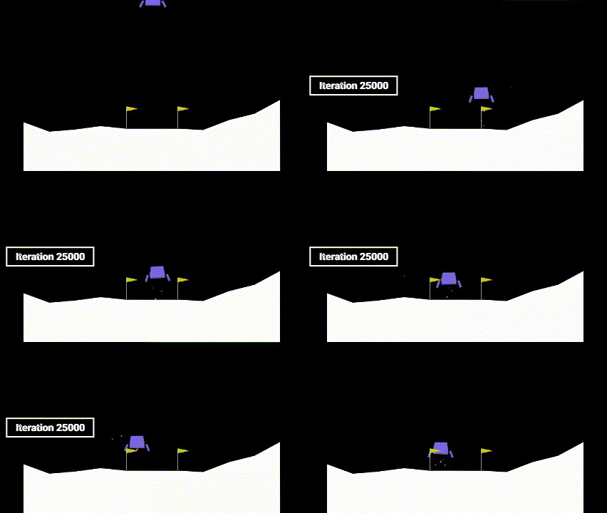 | 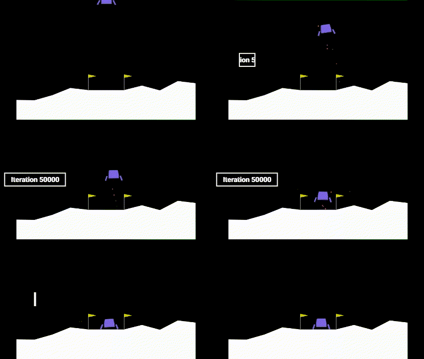 |
As it can be seen, before learning how to land, the agent learns how to hover to prevent crashing. Only after that, it learns how to land.
Evolution Strategy
Evolution Strategy is the simplest algorithm out of the ones implemented in the library. Indeed, the parameters do not need any backpropagation, and a simple estimate of the gradient is computed using perturbations of the parameters. Hence, it does not need any neural network and can be used on any environment, even those with a continuous action space.
To show the results of this technique, I implemented my version of the Flappy Bird game, which can be found in the library.
The model was trained on 200 episodes before achieving a score of 1,000 points, the maximum score I allowed to avoid time-consuming training. At each episode, 30 perturbations of the original model are created to compute the gradient’s estimate. The following plot shows the evolution of the score during training:
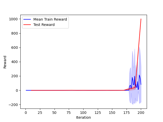
We observe that, once the model starts scoring points, it quickly learns to maximize its score. It makes sense as the difficulty of the game is constant even at high scores, hence the necessity to cap the maximum score.
Here is a showcase of the training of the agent:
| Iteration 0 | Iteration 100 | Iteration 200 |
|---|---|---|
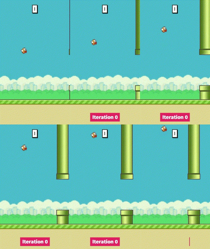 | 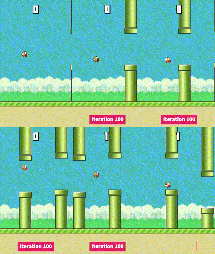 | 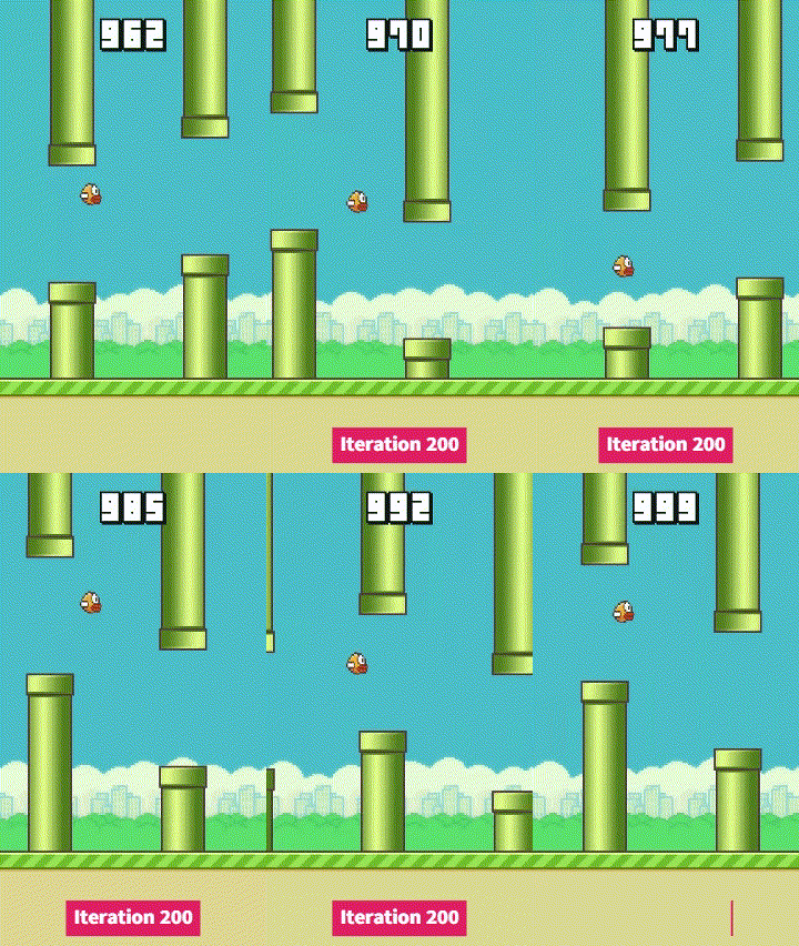 |
We can see that at mid-training, the agent starts to learn how to through a pipe, this is then generalized to more pipes to maximize the score. The video’s speed has been increased on the last iteration to show the agent’s performance.
Deep Deterministic Policy Gradient (DDPG)
I trained a DDPG agent on the HalfCheetah-v4 environment, where a dog-like character must learn to walk forward. The agent was trained on 4,000 episodes on a CPU for 2 hours. The testing rewards look as such:
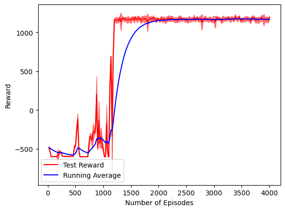
Here the agent suddenly learns how to walk after around 1,200 episodes, and the reward does not increase much after that. This shows that a subtle change in the agent’s behavior has led to a huge improvement in the reward, but that this behavior cannot be much more optimized.
The videos of the agent demonstrate this:
| Iteration 0 | Iteration 1,000 | Iteration 1,200 | Iteration 4,000 |
|---|---|---|---|
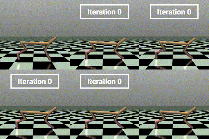 | 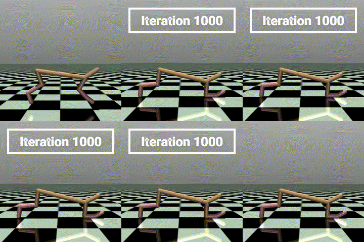 | 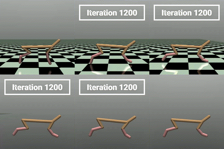 | 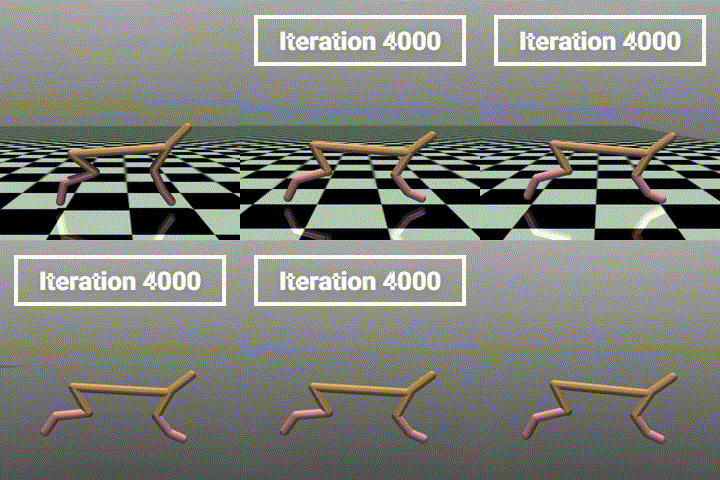 |
We can see that the method adopted by the agent at iteration 1,200 does not evolve much until the end of the training. The agent learns to walk forward, but it does not learn to run, which would be much more efficient. Note that the videos have been accelerated to show the agent’s performance, without acceleration, the agent looks like this:

While the agent goes forward, it is not very efficient compared to state-of-the-art solutions, one can find an example here
Proximal Policy Optimization (PPO)
This algorithm is considered state-of-the-art in RL. It is a policy-based method, meaning that it optimizes the policy directly, rather than optimizing the Q-function. As I discovered when implementing it, a lot of hidden details are needed to make it work efficiently, I found those details on this blog.
To show that my implementation is correct, I trained a PPO agent on the BipedalWalker-v3 environment, where a 2D character must learn to walk. The agent was trained on around 16,000,000 environment steps on a CPU for 5 hours. This was possible thanks to the use of a parallelized environment, which allows to run multiple environments at the same time, and hence to collect more data.
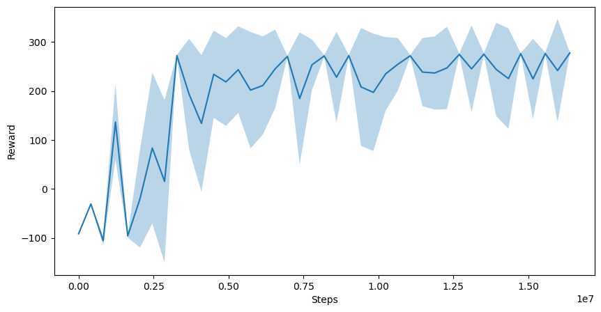
We can see that the agent starts learning how to walk after around 4,000,000 steps, and then improves its performance until it reaches a reward of around 250-300. This is not the maximum reward, but it is already a good performance, and it could be improved with more hyperparameter tuning.
Here is what the agent looks like at different stages of the training:
| Iteration 0 | Iteration 200 | Iteration 400 |
|---|---|---|
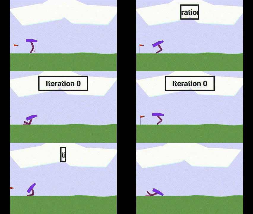 | 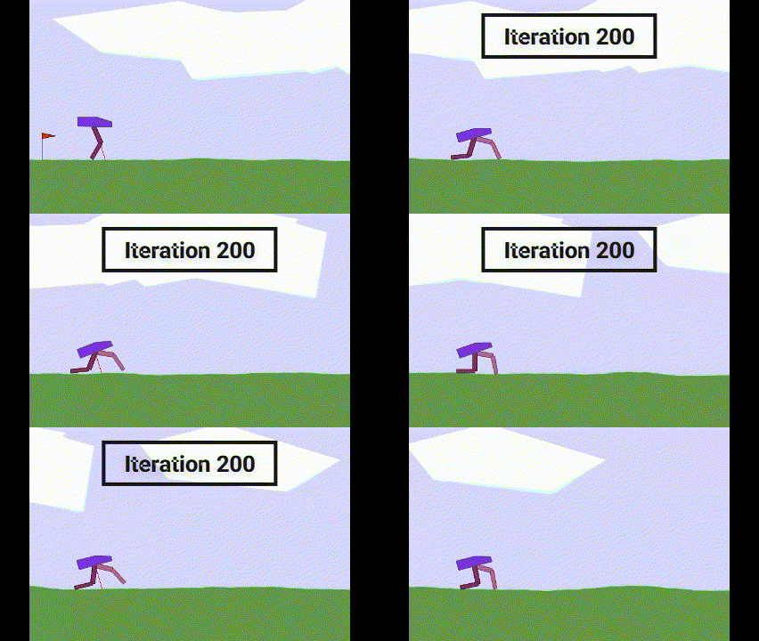 | 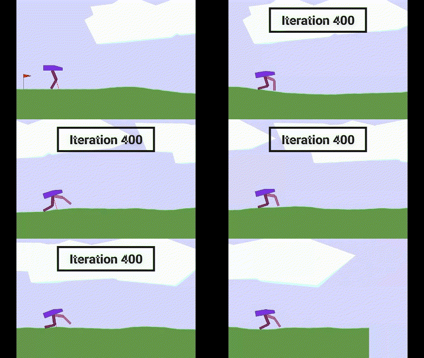 |
Here iteration denotes the number of environment rollouts before updating the model, this is why it is much lower than 16,000,000. We can see that the agent can already go forward at mid-training, by dragging its back knee. At the end of the training, it gets more efficient and its way of walking seems more natural and efficient.
